Table of Contents -- Index -- PS reprint -- PDF reprint

Astronomical Data Analysis Software and Systems VII
ASP Conference Series, Vol. 145, 1998
Editors: R. Albrecht, R. N. Hook and H. A. Bushouse

Noise Detection and Filtering using Multiresolution Transform Methods

Fionn Murtagh (1,2) and Jean-Luc Starck (3)
(1) Faculty of Informatics, University of Ulster, BT48 7JL Derry, Northern Ireland (e-mail fd.murtagh@ulst.ac.uk)
(2) Observatoire Astronomique, 11 rue de l'Université, 67000 Strasbourg Cedex, France (e-mail fmurtagh@astro.u-strasbg.fr)
(3) CEA, DSM/DAPNIA, CE-Saclay, 91191 Gif-sur-Yvette Cedex, France (e-mail jstarck@cea.fr)

 

Abstract:

A new and powerful methodology for treating noise and clutter in astronomical images is described. This is based on the use of the redundant à trous wavelet transform, and the multiresolution support data structure. Variance stabilization and noise modeling are discussed. A number of the examples used in the presentation are shown.

             

1. Introduction

Noise is of fundamental importance in astronomy. In practice we must model it. In this article we present a powerful framework for doing this.

Information on the detector's noise properties may be available (Snyder et al. 1993, Tekalp and Pavlovic 1991). In the case of CCD detectors, or digitized photographic images, additive Gaussian and/or Poisson distributions often provide the most appropriate model.

If the noise model is unknown, e.g., due to calibration and preprocessing of the image data being difficult to model, or having images of unknown detector provenance, or in a case where we simply need to check up on our preconceived ideas about the data we are handling, then we need to estimate noise. An algorithm for automated noise estimation is discussed in Starck and Murtagh (1997).

2. Multiresolution Support

This describes in a logical or boolean way if an image I contains information at a given scale j and at a given position (x,y). If M^(I)(j,x,y) = 1 (or $= \ true$), then I contains information at scale j and at the position (x,y).

M depends on several parameters:

• The input image.
• The algorithm used for the multiresolution decomposition.
• The noise.
• All constraints which we want the support additionally to satisfy.

The multiresolution support of an image is computed in several steps:

• Step 1 is to compute the wavelet transform of the image.
• Booleanization of each scale leads to the multiresolution support.
• A priori knowledge can be introduced by modifying the support.

The last step depends on the knowledge we have of our images. E.g., if no interesting object smaller or larger than a given size in our image, we can suppress, in the support, anything which is due to that kind of object.

3. Multiresolution Support from the Wavelet Transform

The à trous algorithm is described as follows. A pixel at position x,y can be expressed as the sum all the wavelet coefficients at this position, plus the smoothed array:

$$c_0(x,y) = c_{p}(x,y) + \sum_{j=1}^{p} w_j(x,y)$$ (1)

The multiresolution support is defined by:

	M(j,x,y)	= 1	if wj(x,y) is significant	(2)
		= 0	if wj(x,y) is not significant

Given stationary Gaussian noise,

$$\mbox{ if } \mid w_j \mid \ \geq \ k \sigma_j \ \ \mbox{ then } w_j \mbox{ is s significant }$$ (3)

$$\mbox{ if } \mid w_j \mid \ < \ k \sigma_j \ \ \mbox{ then } w_j \mbox{ is not significant }$$

4. Variance Stabilization

We need the noise standard deviation at each scale for iid (independent identically distributed) Gaussian pixel values. In the case of additive Poisson or Poisson plus Gaussian noise, we transform the image so that this is the case. The transform we use is one for variance stabilization.

To compute the standard deviation $\sigma^e_j$ at each scale, simulate an image containing Gaussian noise with a standard deviation equal to 1, and take the wavelet transform of this image.

The standard deviation of the noise at a scale j of the image, $\sigma_j = \sigma_I \sigma^e_j$, where $\sigma_I$ is the standard deviation of the noise in the original image.

If the noise in the data I is Poisson, the transform

$$t(I(x,y)) = 2\sqrt{I(x,y) + \frac{3}{8}}$$ (4)

acts as if the data arose from a Gaussian white noise model, with $\sigma = 1$, under the assumption that the mean value of I is large.

For combined Gaussian and Poisson noise:

$$t(I) = \frac{2}{\alpha} \sqrt{\alpha I(x,y) + \frac{3}{8} \alpha^2 + \sigma^2 - \alpha g}$$ (5)

where $\alpha$ is the gain, $\sigma$ and g the standard deviation and the mean of the read-out noise.

5. Algorithm for Noise Filtering

Reconstruction of the image, after setting non-significant wavelet coefficients to zero, at full resolution provides an approach for adaptive filtering. A satisfactory filtering implies that the error image $E = I - \tilde{I}$, obtained as the difference between the original image and the filtered image, contains only noise and no `structure'. We can easily arrive at this objective by keeping significant wavelet coefficients and by iterating. The following algorithm (Starck et al. 1997) converges quickly to a solution which protects all signal in the image, and assesses noise with great accuracy.

1.

$n \leftarrow 0$.

2.

Initialize the solution, I⁽⁰⁾, to zero.

3.

Determine the multiresolution support of the image.

4.

Estimate the significance level (e.g., 3-sigma) at each scale.

5.

Keep significant wavelet coefficients. Reconstruct the image, I⁽ⁿ⁾, from these significant coefficients.

6.

Determine the error, E⁽ⁿ⁾ = I - I⁽ⁿ⁾ (where I is the input image, to be filtered).

7.

Determine the multiresolution transform of E⁽ⁿ⁾.

8.

Threshold: only retain the coefficients which belong to the support.

9.

Reconstruct the thresholded error image. This yields the image $\tilde{E}^{(n)}$ containing the significant residuals of the error image.

10.

Add this residual to the solution: $I^{(n)} \leftarrow I^{(n)} + \tilde{E}^{(n)}$.

11.

If $\mid (\sigma_{E^{(n-1)}} - \sigma_{E^{(n)}})/\sigma_{E^{(n)}} \mid \ \gt \ \epsilon$ then $n \leftarrow n + 1$ and go to step 4.

6. Example 1: Simulation

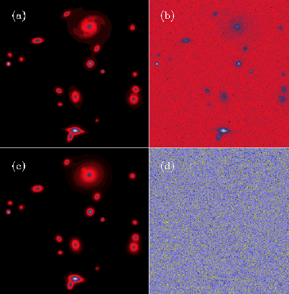
A simulated image containing stars and galaxies is shown in Figure 1 (top left). The simulated noisy image, the filtered image and the residual image are respectively shown in Figure 1 top right, bottom left, and bottom right. We can see that there is no structure in the residual image. The filtering was carried out using the multiresolution support.

  

Figure 1: (a) Simulated image, (b) simulated image and Gaussian noise, (c) filtered image, and (d) residual image.

7. Example 2: Spectrum Filtering

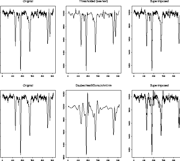
Figure 2 shows a noisy spectrum (upper left, repeated lower right). For the astronomer, the spectral lines - here mainly absorption lines extending downwards - are of interest. The continuum may also be of interest, i.e. the overall spectral tendency.

The spectral lines are unchanged in the filtered version (upper center, and upper right). The lower center (and lower right) version shows the result of applying Daubechies' coefficient 8, a compactly-supported orthonormal wavelet. This was followed by thresholding based on estimated variance of the coefficients, as proposed by Donoho (1990), but not taking into account the image's noise properties as we have done. One sees immediately that a problem- (or image-) driven choice of wavelet and filtering strategy is indispensable.

  

Figure 2: Top row: original noisy spectrum; filtered spectrum using the multiresolution support method; both superimposed. Bottom row: original; filtered (using Daubechies coefficient 8, and Donoho and Johnstone ``universal'' thresholding); both superimposed.

8. Example 3: X-Ray Image Filtering

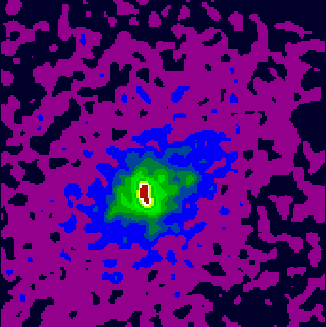
The galaxy cluster A2390 is at a redshift of 0.231. Figure 3 shows an image of this cluster, obtained by the ROSAT X-ray spacecraft. The resolution is one arc second per pixel, with a total number of photons equal to 13506 for an integration time of 8.5 hours. The background level is about 0.04 photons per pixel.

It is obvious that this image cannot be used directly, and some treatment must be performed before any analysis. The standard method consists of convolving the image with a Gaussian. Figure 4 shows the result of such processing. (The Gaussian used had full-width at half maximum equal to 5", which is approximately that of the point spread function). The smoothed image shows some structures, but also residual noise, and it is difficult to give any meaning to them.

Figure 5 shows an image filtered by the wavelet transform (Starck and Pierre 1997a). The noise has been eliminated, and the wavelet analysis indicates faint structures in X-ray emission, allowing explanation of gravitational amplification phenomena, observed in the visible domain (Starck and Pierre 1997b).

  

Figure 3: ROSAT Image of the cluster A2390.

  

Figure 4: ROSAT image of the cluster A2390 filtered by the standard method (convolution by a Gaussian).

  

Figure 5: ROSAT image of the cluster A2390 filtered by the method based on wavelet coefficients.

9. Conclusion

The methods described in this article have been applied to many practical problems over the last few years. A comprehensive treatment of these methods can be found in Starck et al. (1998). A large software package will be available from early 1998.

References:

Donoho, D.L. & Johnstone, I.M. 1993, ``Ideal spatial adaptation by wavelet shrinkage'', Stanford University, Technical Report 400 (available by anonymous ftp from ftp://playfair.stanford.edu/pub/donoho)

Snyder, D.L., Hammoud, A.M. and White, R.L. 1993, J. Optical Soc. Am. 10, 1014

Starck, J.-L. Murtagh, F. & Bijaoui, A. 1998, Image and Data Analysis: the Multiscale Approach, Cambridge University Press, in press

Starck, J.-L. & Murtagh, F. 1997, ``Automatic noise estimation from the multiresolution support'', PASP, in press

Starck, J.-L. & Pierre, M. 1997a, ``X-ray structures in galaxy cores'', to appear in A&A

Starck, J.-L. & Pierre, M. 1997b, ``Structure detection in low intensity X-ray images'', to appear in A&A

Tekalp, A.M. and Pavlovic, G. 1991, in A.K. Katsaggelos, ed., Digital Image Restoration, Springer-Verlag, New York, 209

© Copyright 1998 Astronomical Society of the Pacific, 390 Ashton Avenue, San Francisco, California 94112, USA